.ipynb .pdf

repository open issue suggest edit

Binder Colab

Contents

The \(\chi^2\) Distribution

\(\chi^2\) Test Statistic

If we make \(n\) ranom samples (observations) from Gaussian (Normal) distributions with known means, \(\mu_i\), and known variances, \(\sigma_i^2\), it is seen that the total squared deviation,

\[ \chi^2 = \sum_{i=1}^{n} \left(\frac{x_i - \mu_i}{\sigma_i}\right)^2\,, \]

follows a \(\chi^2\) distribution with \(n\) degrees of freedom.

Probability Distribution Function

The \(\chi^2\) probability distribution function for \(k\) degrees of freedom (the number of parameters that are allowed to vary) is given by

\[ f\left(\chi^2\,;k\right) = \frac{\displaystyle 1}{\displaystyle 2^{k/2} \,\Gamma\left(k\,/2\right)}\, \chi^{k-2}\,e^{-\chi^2/2}\,, \]

where if there are no constrained variables the number of degrees of freedom, \(k\), is equal to the number of observations, \(k=n\). The p.d.f. is often abbreviated in notation from \(f\left(\chi^2\,;k\right)\) to \(\chi^2_k\).

A reminder that for integer values of \(k\), the Gamma function is \(\Gamma\left(k\right) = \left(k-1\right)!\), and that \(\Gamma\left(x+1\right) = x\Gamma\left(x\right)\), and \(\Gamma\left(1/2\right) = \sqrt{\pi}\).

Mean

Letting \(\chi^2=z\), and noting that the form of the Gamma function is

\[ \Gamma\left(z\right) = \int\limits_{0}^{\infty} x^{z-1}\,e^{-x}\,dx, \]

it is seen that the mean of the \(\chi^2\) distribution \(f\left(\chi^2 ; k\right)\) is

\[\begin{split} \begin{align} \mu &= \textrm{E}\left[z\right] = \displaystyle\int\limits_{0}^{\infty} z\, \frac{\displaystyle 1}{\displaystyle 2^{k/2} \,\Gamma\left(k\,/2\right)}\, z^{k/2-1}\,e^{-z\,/2}\,dz \\ &= \displaystyle \frac{\displaystyle 1}{\displaystyle \Gamma\left(k\,/2\right)} \int\limits_{0}^{\infty} \left(\frac{z}{2}\right)^{k/2}\,e^{-z\,/2}\,dz = \displaystyle \frac{\displaystyle 1}{\displaystyle \Gamma\left(k\,/2\right)} \int\limits_{0}^{\infty} x^{k/2}\,e^{-x}\,2 \,dx \\ &= \displaystyle \frac{\displaystyle 2 \,\Gamma\left(k\,/2 + 1\right)}{\displaystyle \Gamma\left(k\,/2\right)} \\ &= \displaystyle 2 \frac{k}{2} \frac{\displaystyle \Gamma\left(k\,/2\right)}{\displaystyle \Gamma\left(k\,/2\right)} \\ &= k. \end{align} \end{split}\]

Variance

Likewise, the variance is

\[\begin{split} \begin{align} \textrm{Var}\left[z\right] &= \textrm{E}\left[\left(z-\textrm{E}\left[z\right]\right)^2\right] = \displaystyle\int\limits_{0}^{\infty} \left(z - k\right)^2\, \frac{\displaystyle 1}{\displaystyle 2^{k/2} \,\Gamma\left(k\,/2\right)}\, z^{k/2-1}\,e^{-z\,/2}\,dz \\ &= \displaystyle\int\limits_{0}^{\infty} z^2\, f\left(z \,; k\right)\,dz - 2k\int\limits_{0}^{\infty} z\,\,f\left(z \,; k\right)\,dz + k^2\int\limits_{0}^{\infty} f\left(z \,; k\right)\,dz \\ &= \displaystyle\int\limits_{0}^{\infty} z^2 \frac{\displaystyle 1}{\displaystyle 2^{k/2} \,\Gamma\left(k\,/2\right)}\, z^{k/2-1}\,e^{-z\,/2}\,dz - 2k^2 + k^2\\ &= \displaystyle\int\limits_{0}^{\infty} \frac{\displaystyle 1}{\displaystyle 2^{k/2} \,\Gamma\left(k\,/2\right)}\, z^{k/2+1}\,e^{-z\,/2}\,dz - k^2\\ &= \frac{\displaystyle 2}{\displaystyle \Gamma\left(k\,/2\right)} \displaystyle\int\limits_{0}^{\infty} \left(\frac{z}{2}\right)^{k/2+1}\,e^{-z\,/2}\,dz - k^2 = \frac{\displaystyle 2}{\displaystyle \Gamma\left(k\,/2\right)} \displaystyle\int\limits_{0}^{\infty} x^{k/2+1}\,e^{-x}\,2\,dx - k^2 \\ &= \displaystyle \frac{\displaystyle 4 \,\Gamma\left(k\,/2 + 2\right)}{\displaystyle \Gamma\left(k\,/2\right)} - k^2 \\ &= \displaystyle 4 \left(\frac{k}{2} + 1\right) \frac{\displaystyle \Gamma\left(k\,/2 + 1\right)}{\displaystyle \Gamma\left(k\,/2\right)} - k^2 \\ &= \displaystyle 4 \left(\frac{k}{2} + 1\right) \frac{k}{2} - k^2 \\ &= k^2 + 2k - k^2 \\ &= 2k, \end{align} \end{split}\]

such that the standard deviation is

\[ \sigma = \sqrt{2k}\,. \]

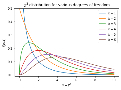
Given this information we now plot the \(\chi^2\) p.d.f. with various numbers of degrees of freedom to visualize how the distribution’s behaviour

import numpy as np
import scipy.stats as stats

import matplotlib.pyplot as plt

# Plot the chi^2 distribution
x = np.linspace(0.0, 10.0, num=1000)

[plt.plot(x, stats.chi2.pdf(x, df=ndf), label=fr"$k = ${ndf}") for ndf in range(1, 7)]

plt.ylim(-0.01, 0.5)

plt.xlabel(r"$x=\chi^2$")
plt.ylabel(r"$f\left(x;k\right)$")
plt.title(r"$\chi^2$ distribution for various degrees of freedom")

plt.legend(loc="best")

plt.show();

Cumulative Distribution Function

The cumulative distribution function (CDF) for the \(\chi^2\) distribution is (letting \(z=\chi^2\))

\[\begin{split} \begin{split} F_{\chi^2}\left(x\,; k\right) &= \int\limits_{0}^{x} f_{\chi^2}\left(z\,; k\right) \,dz \\ &= \int\limits_{0}^{x} \frac{\displaystyle 1}{\displaystyle 2^{k/2} \,\Gamma\left(k\,/2\right)}\, z^{k/2-1}\,e^{-z/2} \,dz \\ &= \int\limits_{0}^{x} \frac{\displaystyle 1}{\displaystyle 2 \,\Gamma\left(k\,/2\right)}\, \left(\frac{z}{2}\right)^{k/2-1}\,e^{-z/2} \,dz = \frac{1}{\displaystyle 2 \,\Gamma\left(k\,/2\right)}\int\limits_{0}^{x/2} t^{k/2-1}\,e^{-t} \,2\,dt \\ &= \frac{1}{\displaystyle \Gamma\left(k\,/2\right)}\int\limits_{0}^{x/2} t^{k/2-1}\,e^{-t} \,dt \end{split} \end{split}\]

Noting the form of the lower incomplete gamma function is

\[ \gamma\left(s,x\right) = \int\limits_{0}^{x} t^{s-1}\,e^{-t} \,dt\,, \]

and the form of the regularized Gamma function is

\[ P\left(s,x\right) = \frac{\gamma\left(s,x\right)}{\Gamma\left(s\right)}\,, \]

it is seen that

\[\begin{split} \begin{split} F_{\chi^2}\left(x\,; k\right) &= \frac{1}{\displaystyle \Gamma\left(k\,/2\right)}\int\limits_{0}^{x/2} t^{k/2-1}\,e^{-t} \,dt \\ &= \frac{\displaystyle \gamma\left(\frac{k}{2},\frac{x}{2}\right)}{\displaystyle \Gamma\left(\frac{k}{2}\right)} \\ &= P\left(\frac{k}{2},\frac{x}{2}\right)\,. \end{split} \end{split}\]

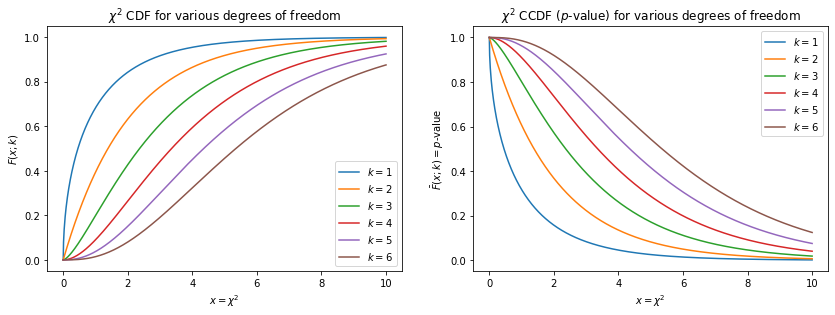
Thus, it is seen that the compliment to the CDF (the complementary cumulative distribution function (CCDF)),

\[ \bar{F}_{\chi^2}\left(x\,; k\right) = 1-F_{\chi^2}\left(x\,; k\right), \]

represents a one-sided (one-tailed) \(p\)-value for observing a \(\chi^2\) given a model — that is, the probability to observe a \(\chi^2\) value greater than or equal to that which was observed.

def chi2_ccdf(x, df):
    """The complementary cumulative distribution function

    Args:
        x: the value of chi^2
        df: the number of degrees of freedom

    Returns:
        1 - the cumulative distribution function
    """
    return 1.0 - stats.chi2.cdf(x=x, df=df)

x = np.linspace(0.0, 10.0, num=1000)
fig, axes = plt.subplots(nrows=1, ncols=2, figsize=(14, 4.5))

for ndf in range(1, 7):
    axes[0].plot(x, stats.chi2.cdf(x, df=ndf), label=fr"$k = ${ndf}")
    axes[1].plot(x, chi2_ccdf(x, df=ndf), label=fr"$k = ${ndf}")

axes[0].set_xlabel(r"$x=\chi^2$")
axes[0].set_ylabel(r"$F\left(x;k\right)$")
axes[0].set_title(r"$\chi^2$ CDF for various degrees of freedom")

axes[0].legend(loc="best")

axes[1].set_xlabel(r"$x=\chi^2$")
axes[1].set_ylabel(r"$\bar{F}\left(x;k\right) = p$-value")
axes[1].set_title(r"$\chi^2$ CCDF ($p$-value) for various degrees of freedom")

axes[1].legend(loc="best")

plt.show();

Binned \(\chi^2\) per Degree of Freedom

TODO

References

• [1] G. Cowan, Statistical Data Analysis, Oxford University Press, 1998

• [2] G. Cowan, “Goodness of fit and Wilk’s theorem”, Notes, 2013

previous

The Gaussian (Normal) Distribution

next

Probability integral transform