Probability integral transform¶

The probability integral transform states that if \(X\) is a continuous random variable with cumulative distribution function \(F_{X}\), then the random variable \(\displaystyle Y=F_{X}(X)\) has a uniform distribution on \([0, 1]\). The inverse of this is the “inverse probability integral transform.’’ [1]

“Proof”¶

Let a random variable, \(Y\), be defined by \(Y = \displaystyle F_{X}(X)\) where \(X\) is another random variable. Then,

\[\begin{split} \begin{split} F_{Y}(y) &= \text{P}(Y \leq y)\\ &= \text{P}(F_{X}(X) \leq y) \\ &= \text{P}(F_{X}(X) \leq F_{X}^{-1}(y)) \\ &= F_{X}(F_{X}^{-1}(y)) \\ &= y. \end{split} \end{split}\]

\(\displaystyle F_{Y}(y) = y\) describes the cumulative distribution function of a random variable, i.e., \(Y = \displaystyle F_{X}(X)\), uniformly distributed on \([0,1]\). [1]

Alternative View: A Change of variables¶

Consider the variable transformation

\[ \begin{equation*} y(x) = F(x) = \int\limits_{-\infty}^{x} f(x')\,dx'. \end{equation*} \]

So the transofrmation from the distribution \(f(x)\) to the distribution \(f(y)\) required a Jacobian (determinant),

\[\begin{split} \begin{split} \frac{dy}{dx} &= \frac{d}{dx} \int\limits_{-\infty}^{x} f(x')\,dx' \\ &= f(x), \end{split} \end{split}\]

such that the distribution of \(y\) is

\[\begin{split} \begin{split} f(y) &= \left(\frac{1}{\left|\frac{dy}{dx}\right|}\right) \,f(x) \\ &= \frac{f(x)}{f(x)}\\ &= 1, \end{split} \end{split}\]

which is the probability density function for the Uniform distribution from \([0,1]\). [2]

Example:¶

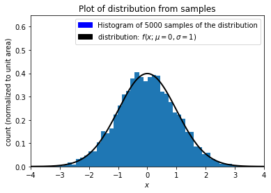
Let’s uniformly sample \(n\) measurements from a Gaussian distribution with true mean \(\mu\) and true standard deviation \(\sigma\).

x = np.linspace(-5.0, 5.0, num=10000)
# mean and standard deviation
mu = 0
sigma = 1

# sample the distribution
number_of_samples = 5000
samples = np.random.normal(mu, sigma, number_of_samples)
samples.sort()

# get sample parameters
sample_mean = np.mean(samples)
sample_std = np.std(samples)

true_distribution = stats.norm.pdf(x, mu, sigma)

Histogram the distribution

n_bins = 1
if number_of_samples < 50:
    n_bins = number_of_samples
else:
    n_bins = 50

# Plots
plt.figure(1)

# Plot histogram of samples
hist_count, bins, _ = plt.hist(
    samples, n_bins, density=True
)  # Norm to keep distribution in view
# Plot distribution using sample parameters
plt.plot(x, true_distribution, linewidth=2, color="black")

# Axes
plt.title("Plot of distribution from samples")
plt.xlabel("$x$")
plt.ylabel("count (normalized to unit area)")
sample_window_w = sample_std * 1.5
# plt.xlim([sample_mean - sample_window_w, sample_mean + sample_window_w])
plt.xlim([-4, 4])
plt.ylim([0, hist_count.max() * 1.6])

# Legends
sample_patch = mpatches.Patch(
    color="black", label=fr"distribution: $f(x;\mu={mu},\sigma={sigma})$"
)
data_patch = mpatches.Patch(
    color="blue",
    label=f"Histogram of {number_of_samples} samples of the distribution",
)

plt.legend(handles=[data_patch, sample_patch])

plt.show()
# print(samples)

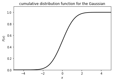
../../_images/probability-integral-transform_22_0.png

Now let’s feed our samples through the cumulative distribution function

# Plots
plt.figure(1)

# Plot distribution using sample parameters
plt.plot(x, stats.norm.cdf(x), linewidth=2, color="black")

# Axes
plt.title("cumulative distribution function for the Gaussian")
plt.xlabel("$x$")
plt.ylabel("$F(x)$")

plt.xlim([-5, 5])
plt.ylim([0, 1.1])

plt.show()

../../_images/probability-integral-transform_24_0.png

output = stats.norm.cdf(samples)
# print(output)

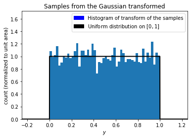
Now let’s plot the output and compare it to the uniform distribution.

# uniform distribution
uniform_distribution = stats.uniform.pdf(x)

# Plots
plt.figure(1)

# Plot histogram of samples
hist_count, bins, _ = plt.hist(
    output, n_bins, density=True
)  # Norm to keep distribution in view
# Plot distribution using sample parameters
plt.plot(x, uniform_distribution, linewidth=2, color="black")
# Axes
plt.title("Samples from the Gaussian transformed")
plt.xlabel("$y$")
plt.ylabel("count (normalized to unit area)")

plt.xlim([-0.25, 1.25])
plt.ylim([0, hist_count.max() * 1.4])

# Legends
sample_patch = mpatches.Patch(
    color="black", label=f"Uniform distribution on $[{0},{1}]$"
)
data_patch = mpatches.Patch(color="blue", label="Histogram of transform of the samples")

plt.legend(handles=[data_patch, sample_patch])

plt.show()

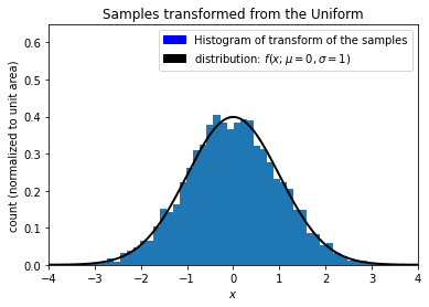
../../_images/probability-integral-transform_28_0.png

Now let’s use the quantile function to recover the original Gaussian distribution from the Uniform distribution.

recovered = stats.norm.ppf(output)

# Plots
plt.figure(1)

# Plot histogram of samples
hist_count, bins, _ = plt.hist(
    recovered, n_bins, density=True
)  # Norm to keep distribution in view
# Plot distribution using sample parameters
plt.plot(x, true_distribution, linewidth=2, color="black")
# Axes
plt.title("Samples transformed from the Uniform")
plt.xlabel("$x$")
plt.ylabel("count (normalized to unit area)")

plt.xlim([-4, 4])
plt.ylim([0, hist_count.max() * 1.6])

# Legends
sample_patch = mpatches.Patch(
    color="black", label=fr"distribution: $f(x;\mu={mu},\sigma={sigma})$"
)
data_patch = mpatches.Patch(color="blue", label="Histogram of transform of the samples")

plt.legend(handles=[data_patch, sample_patch])

plt.show()

../../_images/probability-integral-transform_31_0.png

Summary¶

Thus, we have seen that taking a distribution (pdf) \(X\), and transforming it through the distribution’s cdf will result in an uniform distribution, \(U\), and that transforming \(U\) through the quantile function of \(X\) will result in the pdf of \(X\). Transformations back and forth between \(X\) and \(U\) by careful use of the properties of the cdf and quantile functions is a useful thing to think about. [3]

Statistics Notes

Probability integral transform¶

“Proof”¶

Alternative View: A Change of variables¶

Example:¶

Summary¶

References¶