The Likelihood Function
The joint density of functions of data, \(\vec{x}\), and parameters, \(\vec{\theta}\), is given by their product
Notational Aside:
The notation \( f\left(\vec{x}\,; \vec{\theta}\right) \) is meant to draw attention to the fact that the mulivariable function \(f\) consists of both data and parameters, but that they are fundamentally different quantities. The use of “\(;\)” as the deimlinator
is meant to indicate their difference, but not to imply conditional dependence as “\(|\)” does
Statistical Prediction
If the functions are probability density functions (p.d.f.) then if the parameters, \(\vec{\theta}\), are known, and so fixed, then the probability density to observe the data, \(\vec{x}\), is
As \(p\left(\vec{x} \,\middle|\, \vec{\theta}\right)\) is a probability density function itself, then it is normalizable to unity
Prediction: Using the parameters of interest, \(\vec{\theta}\), and the probability density function to make a statement on the probabily of observing data \(\vec{x}\).
\[ \vec{\theta} \rightarrow f\left(\vec{x} \,\middle|\, \vec{\theta}\right) \rightarrow \vec{x}\]
Statistical Inference
If the data, \(\vec{x}\), have already been observed, and so are fixed, then the joint density is called the “likelihood”. As the data are fixed then the likeilhood is a function of the parameters only
Inference: Using the observed data, \(\vec{x}\), and the likelihood function to make a statement on the compatibility of the parameters of interest, \(\vec{\theta}\), with the observed data.
\[ \vec{x} \rightarrow f\left(\vec{\theta} \,\middle|\, \vec{x}\right) \rightarrow \vec{\theta}\]
Properties of the Likelihood
The likelihood function has proven to be a difficult object to define clearly, as even Fisher only defined it as
“the term […] to designate the state of our information with respect to the parameters of hypothetical populations, and it is shown that the quantitative measure of likelihood does not obey the mathematical laws of probability.” [1]
As the likelihood is a function of the parameters only, then it is seen that it is a function of probability density functions given observed data.
Its values represent the relative compatibility (in some sense) of parameter values with the considered model given the observed data. The greater the value of the likelihood for a parameter value the more compatible the model (with that parameter value) is with the data. There is no sense of an absolute scale of a likelihood (given its formation from an arbitrary number of products of p.d.f.s), but rather its scale is the relative scale of its minimum value and maximum value.
“There is therefore an absolute measure of probability in that the unit is chosen so as to make all the elementary probabilities add up to unity. There is no such absolute measure of likelihood.” [1]
The likelihood is not a probability density. This can most easily be realized by noting that as the likelihood is a function of the parameters only it has no constraint that it is normalized to unity. Indeed, it is not even required to be normalizable. [1,2]
Example: A single sample from the Bernoulli distribution [3]
Given a single observation, \(x\), from the Bernoulli distribution, with probability mass function (p.m.f) (which has \(x \in \{0,1\}\))
sampling \(x=1\) the likelihood is then
As the parameter \(\theta\) for the Bernoulli distribution has range \(0 \leq \theta \leq 1\) (as \(\theta\) represents a probability) then it is seen that
import numpy as np
import matplotlib.pyplot as plt
theta = np.linspace(0.0, 1.0, num=1000)
likelihood = theta

plt.plot(theta, likelihood)

plt.xlabel(r"$\theta$")
plt.ylabel(r"$L\left(\theta | x\right)$")
plt.title(r"Scan in parameter ($\theta$) space of $L\left(\theta | x=1\right)$")

plt.show();
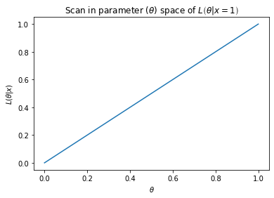
Each point on the above plot is a value of a probability density function given observed data \(\vec{x}\) given the parameter value at that point. The plot itself represents how the value of the probability density of the observed data would change given a scan over the possible parameter values.
Example: The likelihood function for the mean of a Gaussian
The probability distribution function for the Gaussian is
and so the likelihood for data drawn from it is
As this is simulated data (“pseudodata”) it needs to be generated from a “true” distribution.
# mean and standard deviation
true_mu = np.random.uniform(-0.5, 0.5)
true_sigma = np.random.uniform(0.1, 1.0)

print(f"true mean: {true_mu:.3f}")
print(f"true standard deviation: {true_sigma:.3f}")
true mean: -0.105
true standard deviation: 0.260
def gaussian(x, mu, sigma):
    return (
        1 / (sigma * np.sqrt(2 * np.pi)) * np.exp(-((x - mu) ** 2) / (2 * sigma ** 2))
    )


def likelihood(data, parameters):
    return np.prod(gaussian(data, parameters[0], parameters[1]))
The parameter vector is two dimensional, \(\vec{\theta} = \left(\mu, \sigma\right)\), but for the simple case consider fixing the standard deviation such that the likelihood function is a function of a single variable: \(\mu\).
from ipywidgets import interactive
import ipywidgets as widgets
def draw_likelihood(n_samples=100, true_parameters=[true_mu, true_sigma]):
    mu = np.linspace(-1.0, 1.0, num=1000)
    sigma = true_sigma  # only want to be passing in the same value of sigma to the likelihood
    # sample the distribution (which is a Gaussian)
    samples = np.random.normal(true_parameters[0], true_parameters[1], n_samples)

    likelihood_ = np.asarray([likelihood(samples, [mean, sigma]) for mean in mu])
    idx_max_likelihood = np.argmax(likelihood_)

    fig, axes = plt.subplots(nrows=2, ncols=2, figsize=(1.2 * 14, 2.5 * 4.5))

    axes[0, 0].plot(mu, likelihood_, label=r"$L\left(\mu | \vec{x}\right)$")
    axes[0, 0].axvline(
        x=mu[idx_max_likelihood],
        color="black",
        linestyle="--",
        label=fr"$\mu = {mu[idx_max_likelihood]:.3f}$",
    )
    axes[0, 0].axvline(
        x=true_mu,
        color="red",
        linestyle="--",
        label=fr"true $\mu = {true_mu:.3f}$",
    )

    axes[0, 0].set_xlabel(r"$\mu$")
    axes[0, 0].set_ylabel(r"$L\left(\mu | \vec{x}\right)$")
    axes[0, 0].set_title(
        r"Scan in $\mu$ space of $L\left(\mu | \vec{x}\right)$"
        + f" given {n_samples} samples"
    )

    axes[0, 0].legend(loc="best")

    # Repeat for log scale on y-axis
    axes[0, 1].semilogy(mu, likelihood_, label=r"$L\left(\mu | \vec{x}\right)$")
    axes[0, 1].axvline(
        x=mu[idx_max_likelihood],
        color="black",
        linestyle="--",
        label=fr"$\mu = {mu[idx_max_likelihood]:.3f}$",
    )
    axes[0, 1].axvline(
        x=true_mu,
        color="red",
        linestyle="--",
        label=fr"true $\mu = {true_mu:.3f}$",
    )

    # Guard against y-axis scale going off screen
    yaxis_lowest = 10 ** (-300)
    if likelihood_[0] < yaxis_lowest or likelihood_[-1] < yaxis_lowest:
        axes[0, 1].set_ylim(ymin=yaxis_lowest)

    axes[0, 1].set_xlabel(r"$\mu$")
    axes[0, 1].set_ylabel(r"$L\left(\mu | \vec{x}\right)$")
    axes[0, 1].set_title(
        r"Scan in $\mu$ space of $L\left(\mu | \vec{x}\right)$"
        + f" given {n_samples} samples"
    )

    axes[0, 1].legend(loc="best")

    # Show how the sampled data are distributed
    axes[1, 0].plot(mu, likelihood_, label=r"$L\left(\mu | \vec{x}\right)$")
    axes[1, 0].plot(
        samples,
        np.repeat(0, n_samples),
        marker="|",
        color="black",
        linestyle="",
        label=r"$\vec{x}$",
    )

    axes[1, 0].set_xlabel(r"$x$")
    axes[1, 0].set_ylabel(r"$L\left(\mu | \vec{x}\right)$")
    axes[1, 0].set_title(f"Distribution of {n_samples} samples")

    axes[1, 0].legend(loc="best")

    # Hide the 4th plot
    axes[1, 1].axis("off")

    plt.show();
slider_plot = interactive(
    draw_likelihood,
    n_samples=widgets.IntSlider(
        value=50,
        min=1,
        max=200,
        step=1,
        description=r"$n$ samples",
        continuous_update=False,
    ),
    true_parameters=widgets.fixed([true_mu, true_sigma]),
)
display(slider_plot)
To reiterate, this is a plot of a function in parameter space given the observed data.
Given the very distiguishing features of this plot, there is clear motivation to move onto discussions of maximum likelihood esitmators (MLE) in the accompanying notebooks.
References
[1] R. Fisher, “On the Mathematical Foundations of Theoretical Statistics”, Philosophical Transactions of the Royal Society of London. Series A, Containing Papers of a Mathematical or Physical Character, Vol. 222, (1922), pp. 309-368
This is the paper in which Fisher first introduces the idea of the “method of maximum likelihood”.
[2] K. Cranmer, “Practical Statistics for the LHC,” arXiv:1503.07622 [hep-ex].
[3] Cross Validated: What is the reason that a likelihood function is not a pdf?