Unweighted and Weighted Means¶

import numpy as np
import scipy.stats as stats

import matplotlib.pyplot as plt
import matplotlib.patches as mpathces

Maximum Likelihood Estimator motivated “derivations”¶

Unweighted Means¶

If we make \(n\) identical statistically independent (isi) measurements of a random variable \(x\), such that the measurements collected form data \(\vec{x} = \left\{x_i, \cdots, x_n\right\}\), from a Gaussian (Normal) distribution,

\[ \begin{equation} L\left(\vec{x}; \vec{\theta}\right) = \prod_{i=1}^{n} f(x_i; \mu, \sigma) = \frac{1}{(2\pi)^{n/2} \sigma^{n}} \exp\left(-\frac{1}{2\sigma^2} \sum_{i=1}^{n} \left(x_i - \mu\right)^2 \right) \end{equation} \]

then

\[ \begin{equation} -\ln L = \frac{n}{2} \ln\left(2\pi\right) + n \ln \sigma + \frac{1}{2\sigma^2} \sum_{i=1}^{n}\left(x_i - \mu\right)^2 \end{equation} \]

and so \(L\) is maximized with respect to a variable \(\alpha\) when \(-\ln L\) is minimized,

\[ \begin{equation*} \frac{\partial \left(-\ln L\right)}{\partial \alpha} = 0. \end{equation*} \]

Thus, \(L\) is maximized when

\[ \begin{equation*} \frac{\partial \left(-\ln L\right)}{\partial \mu} = -\frac{1}{\sigma^2} \sum_{i=1}^{n}\left(x_i - \mu\right) = 0, \end{equation*} \]

which occurs for

\[ \begin{equation*} \sum_{i=1}^{n} x_i = n \mu, \end{equation*} \]

such that the best estimate for true parameter \(\mu\) is

\[ \begin{equation} \boxed{\hat{\mu} = \frac{1}{n} \sum_{i=1}^{n} x_i = \bar{x}\,}\,, \end{equation} \]

and \(L\) is maximized when

\[ \begin{equation*} \frac{\partial \left(-\ln L\right)}{\partial \sigma} = \frac{n}{\sigma} - \frac{1}{\sigma^3} \sum_{i=1}^{n} \left(x_i - \mu\right) = 0, \end{equation*} \]

which occurs for

\[ \begin{equation*} n\sigma^2 = \sum_{i=1}^{n} \left(x_i - \mu\right)^2, \end{equation*} \]

which is

\[ \begin{equation*} \sigma = \sqrt{\frac{1}{n}\sum_{i=1}^{n} \left(x_i - \mu\right)^2}. \end{equation*} \]

However, \(\mu\) is an unknown true parameter, and the best estimate of it is \(\hat{\mu}\), which is in no manner required to be equal to \(\mu\). Thus, the best estimate of \(\sigma\) is

\[ \begin{equation} \boxed{\hat{\sigma}_{\hat{\mu}} = \sqrt{\frac{1}{n}\sum_{i=1}^{n} \left(x_i - \hat{\mu}\right)^2} = \sqrt{\frac{1}{n}\sum_{i=1}^{n} \left(x_i - \bar{x}\,\right)^2}\,}\,. \end{equation} \]

If the separation from the mean of each observation, \(\left(x_i - \bar{x}\right) = \delta x = \text{constant}\), are the same then the uncertainty on the mean is found to be

\[ \begin{equation*} \sigma_{\hat{\mu}} = \frac{\delta x}{\sqrt{n}}, \end{equation*} \]

which is often referred to as the “standard error”.

So, for a population of measurements sampled from a distribution, it can be said that the sample mean is

\[\mu = \frac{1}{n} \sum_{i=1}^{n} x_i = \bar{x},\]

and the standard deviation of the sample is

\[ \begin{equation*} \sigma = \sqrt{\frac{1}{n}\sum_{i=1}^{n} \left(x_i - \bar{x}\,\right)^2}. \end{equation*} \]

Weighted Means¶

Assume that \(n\) individual measurements \(x_i\) are spread around (unknown) true value \(\theta\) according to a Gaussian distribution, each with known width \(\sigma_i\).

This then leads to the likelihood function

\[ \begin{equation*} L(\theta) = \prod_{i=1}^{n} \frac{1}{\sqrt{2\pi}\sigma_i} \exp\left(-\frac{\left(x_i - \theta\right)^2}{2\sigma_i^2} \right) \end{equation*} \]

and so negative log-likelihood

\[ \begin{equation} -\ln L = \frac{1}{2} \ln\left(2\pi\right) + \ln \sigma_i + \frac{1}{2\sigma_i^2} \sum_{i=1}^{n}\left(x_i - \theta\right)^2. \end{equation} \]

As before, \(L\) is maximized with respect to a variable \(\alpha\) when \(-\ln L\) is minimized,

\[ \begin{equation*} \frac{\partial \left(-\ln L\right)}{\partial \alpha} = 0, \end{equation*} \]

and so \(L\) is maximized with respect to \(\theta\) when

\[ \begin{equation*} \frac{\partial \left(-\ln L\right)}{\partial \theta} = -\sum_{i=1}^{n} \frac{x_i - \theta}{\sigma_i^2} = 0, \end{equation*} \]

which occurs for

\[ \begin{equation*} \sum_{i=1}^{n} \frac{x_i}{\sigma_i^2} = \theta \sum_{i=1}^{n} \frac{1}{\sigma_i^2}, \end{equation*} \]

which is

\[ \begin{equation} \hat{\theta} = \frac{\displaystyle\sum_{i=1}^{n} \frac{x_i}{\sigma_i^2}}{\displaystyle\sum_{i=1}^{n}\frac{1}{\sigma_i^2}}. \end{equation} \]

Note that by defining “weights” to be

\[ \begin{equation*} w_i = \frac{1}{\sigma_1^2}, \end{equation*} \]

this can be expressed as

\[ \begin{equation} \boxed{\hat{\theta} = \frac{\displaystyle\sum_{i=1}^{n} w_i\, x_i}{\displaystyle\sum_{i=1}^{n}w_i}}\,, \end{equation} \]

making the term “weighted mean” very transparent.

To find the standard deviation on the weighted mean, we first look to the variance, \(\sigma^2\). [4]

\[\begin{split} \begin{align*} \sigma^2 &= \text{E}\left[\left(\hat{\theta} - \text{E}\left[\hat{\theta}\right]\right)^2\right] \\ &= \text{E}\left[\left(\frac{\displaystyle\sum_{i=1}^{n} w_i\, x_i}{\displaystyle\sum_{i=1}^{n}w_i} - \text{E}\left[\frac{\displaystyle\sum_{i=1}^{n} w_i\, x_i}{\displaystyle\sum_{i=1}^{n}w_i}\right]\,\right)^2\right] \\ &= \frac{1}{\displaystyle\left(\sum_{i=1}^{n} w_i\right)^2} \text{E} \left[ \displaystyle\left(\sum_{i=1}^{n} w_i\,x_i\right)^2 - 2 \displaystyle\left(\sum_{i=1}^{n} w_i\,x_i\right) \displaystyle\left(\sum_{i=j}^{n} w_j\, \text{E}\left[x_j\right]\right) + \displaystyle\left(\sum_{i=1}^{n} w_i\, \text{E}\left[x_i\right]\right)^2 \right] \\ &= \frac{1}{\displaystyle\left(\sum_{i=1}^{n} w_i\right)^2} \text{E} \left[ \sum_{i,j}^{n} w_i\, x_i w_j\, x_j - 2 \sum_{i,j}^{n} w_i\, x_i w_j\, \text{E}\left[x_j\right] + \sum_{i,j}^{n} w_i\, \text{E}\left[x_i\right] w_j\, \text{E}\left[x_j\right] \right] \\ &= \frac{1}{\displaystyle\left(\sum_{i=1}^{n} w_i\right)^2} \sum_{i,j}^{n} w_i w_j \left( \text{E}\left[ x_i x_j \right] - 2 \text{E}\left[ x_i \right]\text{E}\left[ x_j \right] + \text{E}\left[ x_i \right]\text{E}\left[ x_j \right] \right) \\ &= \frac{1}{\displaystyle\left(\sum_{i=1}^{n} w_i\right)^2} \sum_{i,j}^{n} w_i w_j \left( \text{E}\left[ x_i x_j \right] - \text{E}\left[ x_i \right]\text{E}\left[ x_j \right] \right) \\ &= \frac{1}{\displaystyle\left(\sum_{i=1}^{n} w_i\right)^2} \sum_{i,j}^{n} w_i w_j \,\text{Cov}\left( x_i, x_j \right) = \left\{ \begin{array}{ll} \frac{\displaystyle1}{\displaystyle\left(\sum_{i=1}^{n} w_i\right)^2} \displaystyle\sum_{i}^{n} \left( w_i \sigma_i \right)^2\,, & x_i \text{ and } x_j \text{ statistically independent}, \\ 0\,, &\text{ otherwise}, \end{array} \right. \\ &= \frac{\displaystyle\sum_{i}^{n} \left( \sigma_i^{-2} \sigma_i \right)^2}{\displaystyle\left(\sum_{i=1}^{n} w_i\right)^2} = \frac{\displaystyle\sum_{i}^{n} w_i}{\displaystyle\left(\sum_{i=1}^{n} w_i\right)^2} \\ &= \frac{\displaystyle 1}{\displaystyle\sum_{i=1}^{n} w_i} \end{align*} \end{split}\]

Thus, it is seen that the standard deviation on the weighted mean is

\[ \begin{equation} \boxed{\sigma_{\hat{\theta}} = \sqrt{\frac{\displaystyle 1}{\displaystyle\sum_{i=1}^{n} w_i}} = \left(\displaystyle\sum_{i=1}^{n} \frac{1}{\sigma_i^2}\right)^{-1/2}}\,. \end{equation} \]

Notice that in the event that the uncertainties are uniform for each observation, \(\sigma_i = \delta x\), the above yields the same result as the unweighted mean. \(\checkmark\)

After this aside it is worth pointing out that [1] have a very elegant demonstration that

\[ \begin{equation*} \sigma_{\hat{\theta}} = \left(\frac{\partial^2\left(- \ln L\right)}{\partial\, \theta^2}\right)^{-1/2} = \left(\displaystyle\sum_{i=1}^{n} \frac{1}{\sigma_i^2}\right)^{-1/2}. \end{equation*} \]

So, the average of \(n\) measurements of quantity \(\theta\), with individual measurements, \(x_i\), Gaussianly distributed about (unknown) true value \(\theta\) with known width \(\sigma_i\), is the weighted mean

\[ \begin{equation*} \hat{\theta} = \frac{\displaystyle\sum_{i=1}^{n} w_i\, x_i}{\displaystyle\sum_{i=1}^{n}w_i}, \end{equation*} \]

with weights \(w_i = \sigma_i^{-2}\), with standard deviation on the weighted mean

\[ \begin{equation*} \sigma_{\hat{\theta}} = \sqrt{\frac{\displaystyle 1}{\displaystyle\sum_{i=1}^{n} w_i}} = \left(\displaystyle\sum_{i=1}^{n} \frac{1}{\sigma_i^2}\right)^{-1/2}. \end{equation*} \]

Specific Examples¶

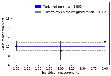
Given the measurements

\[ \vec{x} = \left\{10, 9, 11\right\} \]

with uncertanties

\[\vec{\sigma_x} = \left\{1, 2, 3\right\}\]

x_data = [10, 9, 11]
x_uncertainty = [1, 2, 3]

numerator = sum(x / (sigma_x ** 2) for x, sigma_x in zip(x_data, x_uncertainty))
denominator = sum(1 / (sigma_x ** 2) for sigma_x in x_uncertainty)

print(f"hand calculated weighted mean: {numerator / denominator}")

hand calculated weighted mean: 9.897959183673468

Using NumPy’s average method

# unweighted mean
np.average(x_data)

10.0

x_weights = [1 / (uncert ** 2) for uncert in x_uncertainty]
# weighted mean
weighted_mean = np.average(x_data, weights=x_weights)
print(weighted_mean)

9.897959183673468

# no method to do this in NumPy!?
sigma = np.sqrt(1 / np.sum(x_weights))
print(f"hand calculated uncertaintiy on weighted mean: {sigma}")

hand calculated uncertaintiy on weighted mean: 0.8571428571428571

# A second way to find the uncertainty on the weighted mean
summand = sum((x * w) for x, w in zip(x_data, x_weights))
np.sqrt(np.average(x_data, weights=x_weights) / summand)

0.8571428571428571

Let’s plot the data now and take a look at the results

def draw_weighted_mean(data, errors, w_mean, w_uncert):
    plt.figure(1)

    # the data to be plotted
    x = [i + 1 for i in range(len(data))]

    x_min = x[x.index(min(x))]
    x_max = x[x.index(max(x))]

    y = data
    y_min = y[y.index(min(y))]
    y_max = y[y.index(max(y))]

    err_max = errors[errors.index(max(errors))]

    # plot data
    plt.errorbar(x, y, xerr=0, yerr=errors, fmt="o", color="black")
    # plot weighted mean
    plt.plot((x_min, x_max), (w_mean, w_mean), color="blue")
    # plot uncertainty on weighted mean
    plt.plot(
        (x_min, x_max),
        (w_mean - w_uncert, w_mean - w_uncert),
        color="gray",
        linestyle="--",
    )
    plt.plot(
        (x_min, x_max),
        (w_mean + w_uncert, w_mean + w_uncert),
        color="gray",
        linestyle="--",
    )

    # Axes
    plt.xlabel("Individual measurements")
    plt.ylabel("Value of measruement")
    # view range
    epsilon = 0.1
    plt.xlim(x_min - epsilon, x_max + epsilon)
    plt.ylim([y_min - err_max, 1.5 * y_max + err_max])

    # ax = figure().gca()
    # ax.xaxis.set_major_locator(MaxNLocator(integer=True))

    # Legends
    wmean_patch = mpathces.Patch(
        color="blue", label=fr"Weighted mean: $\mu={w_mean:0.3f}$"
    )
    uncert_patch = mpathces.Patch(
        color="gray",
        label=fr"Uncertainty on the weighted mean: $\pm{w_uncert:0.3f}$",
    )
    plt.legend(handles=[wmean_patch, uncert_patch])

    plt.show()

draw_weighted_mean(x_data, x_uncertainty, weighted_mean, sigma)

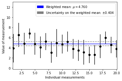
Now let’s do this again but with data that are Normally distributed about a mean value

true_mu = np.random.uniform(3, 9)
true_sigma = np.random.uniform(0.1, 2.0)
n_samples = 20

samples = np.random.normal(true_mu, true_sigma, n_samples).tolist()
gauss_errs = np.random.normal(2, 0.4, n_samples).tolist()

weights = [1 / (uncert ** 2) for uncert in gauss_errs]

draw_weighted_mean(
    samples,
    gauss_errs,
    np.average(samples, weights=weights),
    np.sqrt(1 / np.sum(weights)),
)

References¶

Data Analysis in High Energy Physics, Behnke et al., 2013, \(\S\) 2.3.3.1
Statistical Data Analysis, Glen Cowan, 1998
University of Marlyand, Physics 261, Notes on Error Propagation
Physics Stack Exchange, How do you find the uncertainty of a weighted average?

Statistics Notes

Unweighted and Weighted Means¶

Maximum Likelihood Estimator motivated “derivations”¶

Unweighted Means¶

Weighted Means¶

Specific Examples¶

References¶